Pattern formation in simple systems
02/08/2015
c++, mathematics, python
Last summer, together with a colleague I held an introductory course in the programming language Python at the University of Münster where the participents were especially taught in the basics of numerical programming with this language. At that time I stumbled over a paper by J. E. Pearson (1993) in which a mathematical model for pattern formation in biological systems was presented that despite its relative simplicity is able to produce a variety of complex dynamics. Since the implementation is already possible with the means presented within the course I presented it as a motivating example in the end. Months had passed until this week I read an article at Spiegel online (a german newsportal) where a paper (Stoop et al., 2014) about a model for pattern formation on elastic surfaces was described. Because the images presented therein had strong similarities with my own simulations I decided to make an article about it.
Modelling and numerical ansatz
This section is devoted to a short demonstration of the modelling and the basics of the numerical treatment and is thought for the mathematically experienced readers of this blog. Anyone else who is just interested in the fancy images and videos may jump forward to the next second.
The model presented in Pearson's paper "Complex Patterns in a Simple System" is based on the chemical reaction of two different species whose contentrations will be denoted by $U(t)$ and $V(t)$. The fundamental reaction equations are the following:
$$
    \begin{align*}
        U + 2V &\to 3V \\
            V &\to P
    \end{align*}
$$
Vividly speaking this means that one part of substance $U$ reacts with two parts of $V$ to form three part of $V$, while $V$ itself decomposes into a further product $P$. This is why we call $U$ the activator, because it allows the reaction to happen in the first place. It is also clear that $U$ has to be refilled continuously to keep the reaction going.
From this reaction equations we can deduce a mathematical model for the concentrations $U(t)$ and $V(t)$. This leads to the following system of partial differential equations:
$$
    \begin{align*}
        \partial_t U(t) &= D_U \Delta U(t) - U(t) V^2(t) + F(1 - U(t)) \\
        \partial_t V(t) &= D_V \Delta V(t) + U(t) V^2(t) - (F+k) V(t)
    \end{align*}
$$
together with periodic boundary conditions. The parameters are the diffusion constants $D_U, D_V$, a feed rate $F$ and a reaction rate $k$ of the second equation relative to the first one. As we can see this is a coupled system of reaction-diffusion equations. This system is numerically very stable so that a simple explicit Euler scheme for the time discretization together with finite difference in space is good enough to do the simulations. The explicit time stepping scheme has the advantage that no cumbersome decoupling mechanism is needed. For the step sizes taking both $\Delta t$ and $\Delta h$ as 1 is sufficient. As computational domain we use $[0,N]^2$ for an integer $N$ which is typically taken as 256 or 512. For the simulations, both diffusion constants were fixed while both the feed rate an the reaction rate could be changed. For the images and videos the concentration profile $V(t)$ was used.
Simulation results
Since the simulation speed of the original Python implementation was not satisfactory for me I decided to re-implement it in C++ using the Qt framework. The source code of both programs can be found on my Github account under github.com/michaelschaefer/grayscott. The results presented here were created using the C++ version, a screenshot of which is shown here:
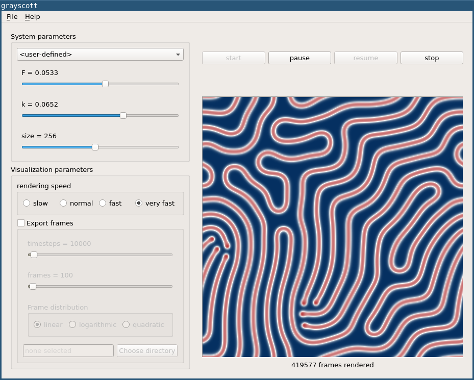 The program allows to vary the relevant model parameters as well as the resolution of the resulting images. Additionally, sequences of images can automatically be saved to disk so that they can be converted into videos by a suitable tool. Although the system dynamics reacts very sensitively to changes in the parameters we can essentially distinguish three categories each of which is presented below, together with some simulation results. By clicking the images you get to the associated video file.
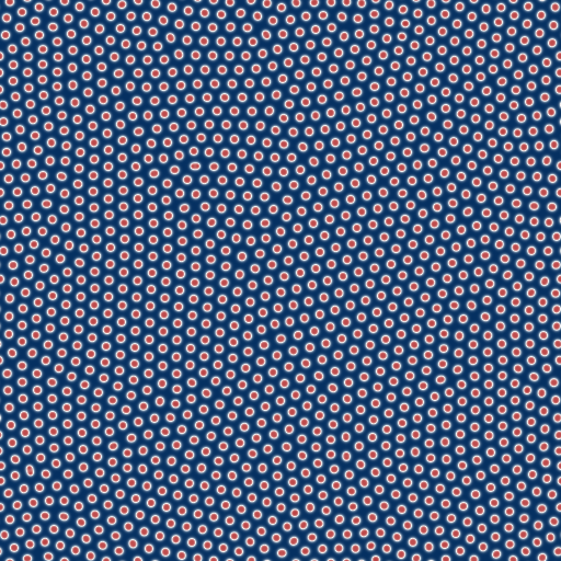
- bacteria-like patterns (even with cell division!) consisting of individual, stationary or barely moving points (F=0.035, k=0.065, N=512. Video size: 2,4MB)
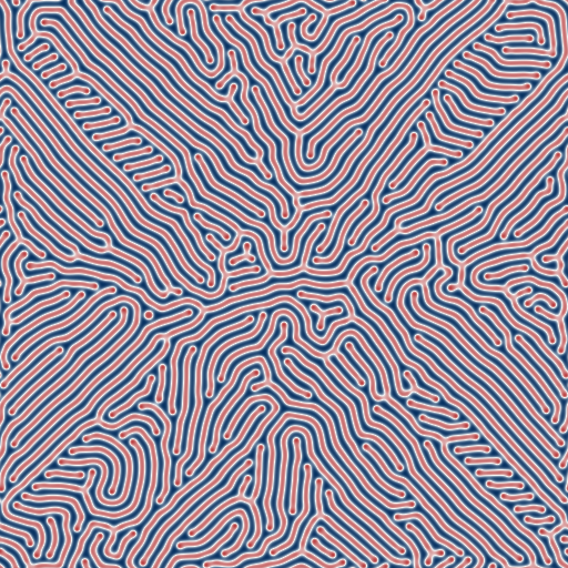
- fingerprint-like patterns made of many convoluted lines (F=0.035, k=0.06, N=512. Video size: 2.5MB)
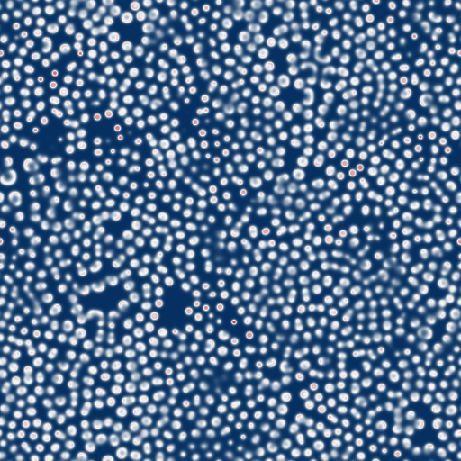
- chaotic patterns of permanently appearing and disappearing points (F=0.02, k=0.055, N=512. Video size: 8.9MB)
As an additional gimmick I have create a kind of map of this model by the following procedure: First, simulations were run for a variety of different values for the parameters F and k. After some time a (hopefully) representative image for the particular dynamics was taken. In the end, all these images were stitched together to a large image, the map. All in all, 81 different values for F and 41 for k were used so that the final map consists of 3,321 individual images. Calculations took several hours on a multi-core system. Though using JPEG compression, the image is still about 3.6MB in size, so that I decided not to integrate it directly but just placing a link to it. The values of F are constant in each row while k stays the same along the columns.